Explainable Boosted Scoring
Introducing the xbooster Library: A Novel Approach to Credit Risk Modeling
Today’s world of financial products is ever evolving, and the ability to develop and validate accurate credit risk models is more important than ever. Whether you’re a data scientist, risk manager, or part of a banking team responsible for credit risk work, understanding and communicating the inner workings of predictive models is crucial. Business knowledge and model interpretability are key pillars of model development in this domain, especially when it comes to communicating model insights to users, regulators, and auditors.
The xbooster library is a modeling toolkit designed for credit risk model developers and validators. Born from research on machine learning (ML) in the area of Credit Risk, the concept was first introduced in Paul Edwards’ NVIDIA GTC talk, Machine Learning in Retail Credit Risk. The concept of boosted scorecards discussed in the talk inspired this library, enabling you to build credit scorecards that can challenge the baseline of Weight of Evidence (WOE) logistic regression.
Understanding the Baseline: Logistic Regression in Credit Risk
In credit risk, the most common prediction task is assessing the probability of default, which measures how likely a customer is to repay a loan. The preferred model for this assessment is logistic regression, a highly mature statistical method renowned for its effectiveness in predicting default probabilities (it’s a direct probability model according to Frank Harrell).
In many retail credit models, logistic regression is complemented with a Weight of Evidence (WOE) layer that allows to introduce a Naive Bayes element into the model and helps to easily construct a credit scorecard from the resulting pipeline.
You can read more about WOE in the blog below:
What is a credit scorecard?
A credit scorecard can be understood a logarithmic points system, that allows to convert model predictions into a numerical range in a desired interval (e.g., from 100 to 600). A high credit score for a given group indicates a lower risk of default, and conversely, a low score suggests higher risk. The groups (bins or risk buckets) which are shown below are commonly obtained using a combination of statistical tools (e.g., decision trees or libraries like OptBinning) and business judgment.
The example below illustrates a simplified scorecard that considers two key risk factors: past loan delinquencies and credit card usage.

Note: If a customer has no past delinquencies and low credit line usage, they will receive 46 points (21 + 25). Alternatively, if the customer has a history of delinquencies and is maxing out the card limit, the customer will get 0 points.
Scorecards can include many more features because they are additive; we simply combine evidence from various features into the final prediction. This makes them easy to understand, communicate, and deploy using SQL alone.
What are credit scores?
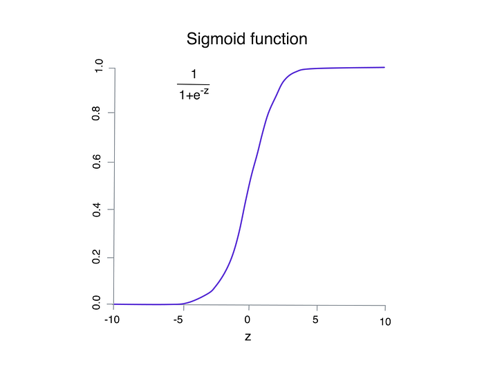
Credit scores reflect the odds of a customer being a “good” or “bad” credit risk. If you’re familiar with binary classification problems involving “good/bad” events, you may recognize the sigmoid function that maps log-odds values onto a probability scale. Logistic regression is linear in log-odds, so converting the logit (z) to probability (p) requires using the sigmoid function, typically handled automatically by logistic regression software.
The scorecard point system directly uses the logit score (z) when applying the Points to Double Odds (PDO) method. This requires three parameters:
- Target points: e.g., 600
- Target odds: e.g., 20 to 1
- Points to double the odds (PDO): e.g., 50
A target points of 600 represents odds of 20 to 1 (P(“good”)/P(“bad”) = 20), and the PDO parameter ensures that moving across WOE groups doubles the odds. The parameters are usually selected based on expert judgment.
If you are new to the topic and want to learn more about building WOE logistic regression scorecards, check out this blog:
Can we improve the baseline with ML?
A scorecard is a binned, additive version of logistic regression. Gradient boosting classification algorithms also perform a version of additive logistic regression, as outlined in the seminal paper (FHT 2000).
Paul Edwards’ NVIDIA talk showed that you can directly generate scorecards with boosting algorithms, gaining accuracy without sacrificing explainability. When properly constrained, boosted scorecards are indistinguishable from traditional scorecards. They are easy to build, robust to multicollinearity, and typically perform a few percentage points better than traditional scorecards.
The xbooster library implements and extends this methodology using the XGBoost algorithm for logistic regression. XGBoost was chosen for its resemblance to the traditional implementation of GBM by J. Friedman and its excellent parsing functionality, which makes it an ideal candidate for credit risk models.
Getting started ⤵

We can install the xbooster library using pip. You can also add xbooster to your poetry environment with poetry add xbooster.
pip install xboosterWe’ll need some data to showcase the library in action. To do this, we’ll use a credit dataset containing examples of both good and bad credit risk performance. Several features will be used to predict the performance of loan accounts within the next 24 months (good means there will be no default and bad means there will be default).
import pandas as pd
from sklearn.model_selection import train_test_split

# Fetch blended credit data
url = (
    "https://github.com/xRiskLab/xBooster/raw/main/examples/data/credit_data.parquet"
)
dataset = pd.read_parquet(url)

features = [
    "external_risk_estimate",
    "revolving_utilization_of_unsecured_lines",
    "account_never_delinq_percent",
    "net_fraction_revolving_burden",
    "num_total_cc_accounts",
    "average_months_in_file",
]

target = "is_bad"

X, y = dataset[features], dataset[target]

ix_train, ix_test = train_test_split(
    X.index, stratify=y, test_size=0.3, random_state=62
)
Next we will fit an XGBoost logistic regression model with a depth of 1 (stumps). min_child_weight parameters allows us to control the overfitting behavior of the model.
import numpy as np
import xgboost as xgb
from sklearn.metrics import roc_auc_score

best_params = dict(
    n_estimators=100,
    learning_rate=0.55,
    max_depth=1,
    min_child_weight=10,
    grow_policy="lossguide",
    early_stopping_rounds=5
)

# Create an XGBoost model
xgb_model = xgb.XGBClassifier(
    **best_params, random_state=62
)
evalset = [
    (X.loc[ix_train], y.loc[ix_train]),
    (X.loc[ix_test], y.loc[ix_test])
]

# Fit the XGBoost model
xgb_model.fit(
    X.loc[ix_train],
    y.loc[ix_train],
    eval_set=evalset,
    verbose=False
)
Scorecard constructor 🗃️️
Now we can create a scorecard with xbooster. First, we instantiate the XGBScorecardConstructor class from the constructor module and generate scorecard points. The scaling parameters pdo of 50, target_points of 600, and target_odds of 50 were chosen arbitrarily. Finally, credit_scores contains the credit scores.
from xbooster.constructor import XGBScorecardConstructor
# Set up the scorecard constructor
scorecard_constructor = XGBScorecardConstructor(
xgb_model, X.loc[ix_train], y.loc[ix_train]
)
# Construct the scorecard
xgb_scorecard = scorecard_constructor.construct_scorecard()
# Create scorecard points
xgb_scorecard_with_points = (
scorecard_constructor.create_points(
pdo=50, target_points=600, target_odds=50
)
)
# Make predictions using the scorecard
credit_scores = scorecard_constructor.predict_score(
X.loc[ix_test]
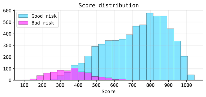
)We can use the explainer module to visualize the resulting distribution of scores. We will see that a good cut-off would lie around between 400 and 500 to separate good and bad credit risk.
from xbooster.explainer import plot_score_distribution

# Plot score distribution
plot_score_distribution(
    scorecard_constructor=scorecard_constructor,
    fontsize=11,
    figsize=(8, 3),
    dpi=600
)
We can look at xgb_scorecard_with_points more closely. Essentially, it's a pandas DataFrame containing information about splits made by decision trees in a gradient-boosted tree model, along with additional metrics not readily available directly from XGBoost.
In this step, we make a subset of the scorecard by selecting only the first three trees (consider these as sub-models):
df = xgb_scorecard_with_points.query("Tree < 3")
display(df)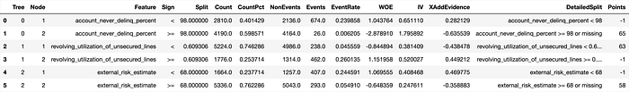
By inspecting the DataFrame above, you’ll notice summary statistics of splits, such as the count of observations or event rate. Additionally, it shows Weight of Evidence (WOE) and Information Value (IV), which are well known to credit risk model developers. The XAddEvidence column represents the raw prediction (classification margin) of XGBoost, which is conceptually similar to WOE. The DetailedSplit column is crucial for XGBoost models with depths greater than 1.
We can also plot these trees, showing the metrics we’re interested in. For example, here’s the tree with index 2 (the third iteration of gradient boosting):
from xbooster.explainer import TreeVisualizer
from matplotlib import pyplot as plt

tree_viz = TreeVisualizer(
    metrics=["Points", "Count"], precision=2
)

tree_id = 2

plt.figure(figsize=(6, 3), dpi=600)
tree_viz.plot_tree(scorecard_constructor, num_trees=tree_id)
plt.title(f"Boosted Scorecard Tree {tree_id}", fontsize=16)
plt.show()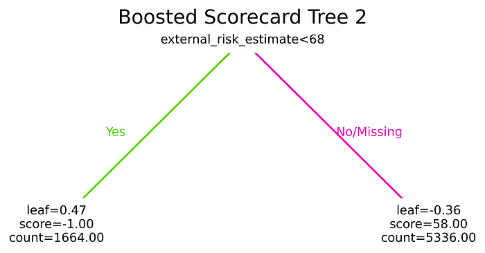
We can see that the data in the tree diagram reflects the data from xgb_scorecard_with_points for the tree with index 2. If external credit risk marker is below 68 points, we assume high risk and assign -1 as a credit score for this feature.
We can serialize the boosted scorecard as follows:
import pickle

with open("models/scorecard_constructor.pkl", "wb") as f:
    pickle.dump(scorecard_constructor, f)
Interpretability 🎐
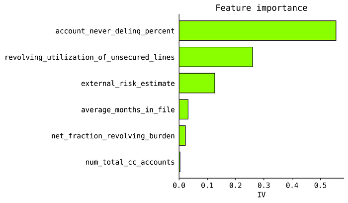
We can gauge overall feature importance with plot_importance method. Several other metrics are available instead of IV.
from xbooster.explainer import plot_importance

plot_importance(
    scorecard_constructor,
    metric="IV",
    method="global",
    normalize=True,
    color="#a7fe01",
    edgecolor="#1e1e1e",
    figsize=(3, 3),
    dpi=200,
    title="Feature importance"
)
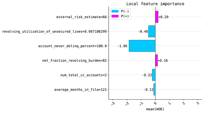
In case we are interested in a single example, we can also plot local explanations with plot_local_importance method.
from xbooster import explainer

# Choose a sample
sample_idx = 2

explainer.plot_local_importance(
    scorecard_constructor,
    X.loc[ix_test][sample_idx : sample_idx + 1],
    figsize=(7, 4),
    fontsize=14,
    dpi=200,
    title="Local feature importance"
)
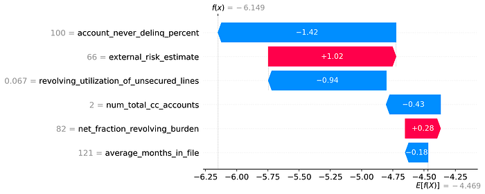
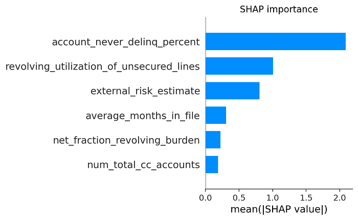
The results from global and local importance methods are highly consistent with TreeSHAP, both for stumps and trees with a depth larger than one. However, xbooster does not require any complex calculations since the scorecard DataFrame contains all the required information about metrics that practitioners can understand from the context of traditional scorecards.
For trees with a depth larger than one, the interpretability is achieved by extending the framework to all individual splits created in a tree branch. For example, if two features were used in a splitn, we will need to calculate statistics (such as counts and event rates) for each individual split condition of each feature. This information about split conditions is stored in DetailedSplit column in the scorecard DataFrame. We invite the reader to learn more about this approach here.
I hope it was well worth your time! 👩💻
Repo, distribution, and docs ⤵
▹ Link to GitHub: https://github.com/xRiskLab/xBooster
▹ Link to PyPI: https://pypi.org/project/xbooster/
▹ Link to Docs: https://xrisklab.ai/
If you would like to access the code used in this example, you can find it in this colab notebook. If you are interested in more use cases, please have a look at some of the other examples of usage in the repo’s \examples.
You can also read more about this library here with a bit less technical explanation and tutorials, which include:
- Customized tree visualization
- Working with categorical data using a preprocessor and
interaction_constraintsparameter - SQL deployment using DuckDB
Additional resources 📚
Below you can find some useful resources about scorecard boosting through presentations, blogs and other projects.
Gradient boosting 📉
- How to Explain Gradient Boosting
- Understanding Gradient Boosting as a Gradient Descent
- Around Gradient Boosting: Classification, Missing Values, Second Order Derivatives, and Line Search
- How Does Extreme Gradient Boosting (XGBoost) Work?
Scorecard boosting 💳
- Boosting for Credit Scorecards and Similarity to WOE Logistic Regression
- Machine Learning in Retail Credit Risk: Algorithms, Infrastructure, and Alternative Data — Past, Present, and Future
- Building Credit Risk Scorecards with RAPIDS
- XGBoost for Interpretable Credit Models
- credit_scorecard — Project
- vehicle_loan_defaults — Artifacts 📊
Thank you for reading through the post! 🙇♂️ If you enjoyed this article, don’t forget to clap 👏.
Below are some additional links:
▹ GitHub: https://github.com/deburky
▹ LinkedIn: https://www.linkedin.com/in/denisburakov
▹ My e-book project on Credit Risk Modeling: https://risk-practitioner.com
▹ My Portfolio of Risk & ML projects: https://linktr.ee/deburky
—
What’s your take on the integration of machine learning with traditional financial models? Have you worked with similar tools? Share your thoughts and experiences in the comments below!