WoeBoost: A Boosted Scoring System
Towards interpretable, evidence-driven scoring models

The evolution of machine learning (ML) algorithms for tabular data has been closely tied to advancements in gradient boosting methodology. From Jerome Friedman’s pioneering work on Gradient Boosting Machines (GBM) in the early 2000s, to XGBoost’s breakthrough in 2016, and more recently CatBoost, gradient boosting has become the go-to solution for tabular problems.
At the same time, while gradient boosted trees have gained adoption in non-regulated industries, it has not seen the same level of interest in fields like finance. This is largely because existing algorithms — such as logistic regression models, which have been in use for decades — are often better suited for the task at hand. These models are statistically sound, interpretable, and align with regulatory requirements.
Additionally, the inner workings of gradient boosting trees are something of a mystery to the typical user. Even relatively established techniques like SHAP values — intended to explain these models — don’t provide the exact rigor that model users and validators expect. For validators and regulators, gradient-boosted trees cannot easily be kept within the guardrails of traditional statistical tests and validation frameworks.
In this post, I introduce WoeBoost, a Python package designed to bridge this gap by presenting gradient boosting in a credit scoring framework. WoeBoost uses the principles of Weight of Evidence (WOE), while drawing on the history of ideas from Harold Jeffreys, Alan Turing, and Jack Good. This package is a sequel to my earlier development of xBooster, a Python package for building explainable scorecards using XGBoost.
Origins of Scoring Systems
Weight of Evidence (WOE) is a concept that often surprises those who aren’t familiar with the world of lending and credit risk (and let’s be honest, it isn’t widely appreciated outside the industry).
Many perceive WOE as a preprocessing technique to:
- Linearize inputs for logistic regression modeling,
- Handle missing values, or
- Encode business rules (e.g., ensuring certain features align with intuition, such as higher income being negatively associated with credit default).
In reality, Weight of Evidence is far more than just a preprocessing tool. It is an inference framework based on likelihood ratios, first formally recognized by Charles S. Peirce in an 1878 essay. Peirce described WOE as the logarithm of chance — what we now refer to as log odds.
The idea is tightly connected to the odds form of Bayes’ Theorem, first discovered, presumably, by Harold Jeffreys. In this form, the posterior probability is proportional to the prior probability times the likelihood, which translates into log odds + evidence (or support) in logarithmic terms.
Perhaps the most fascinating and least appreciated aspect of WOE is its connection to Alan M. Turing. While Turing never explicitly referred to “Weight of Evidence,” he used the closely related concept of log factors to describe independent pieces of evidence supporting a theory.
In one of his declassified wartime papers from the 1940s, Turing introduced the Factor Principle, essentially Bayes’ Theorem, describing “the factor for the theory on account of the data” — precisely what WOE represents.
Turing relied heavily on the log factors in his cryptography work at Bletchley Park, laying the groundwork for modern scoring systems. His methods allowed for evidence to be combined additively, paving the way for interpretable models like those used in credit scoring today.

Turing’s Factor Principle
Log factors (WOE) represent the strength of evidence in favor of or against a theory, based on independent pieces of evidence derived from data.
Weight of Evidence (WOE) quantifies the strength of evidence supporting or refuting a theory, derived from independent pieces of data. Alan M. Turing explored this concept in his wartime work, introducing what he called the Factor Principle — essentially a logarithmic version of Bayes’ Theorem. Below, I summarize Turing’s perspective on scoring using log-factors (WOE) from Chapter 1 of his declassified paper.
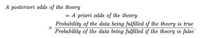
The ratio above is the likelihood ratio, which Turing calls “the factor for the theory on account of the data.” It later became known as the Bayer factor.
In the example from the paper Turing provides, the theory is that the man died of heart failure, and the data is that he died in his bed. Turing provides statistics for this scenario:
Evidence in favor of the theory (heart failure):
- 2/3 of men who die of heart failure die in their beds
- 2/5 . . . . . . . . . . . . . . . . . . . . . . . . . . . . . . . . . have fathers who died of heart failure
- 1/2 . . . . . . . . . . . . . . . . . . . . . . . . . . . . . . . . . have bedroom on the ground floor
Evidence against the theory (other causes):
- 1/4 of men who died from other causes die in their beds
- 1/6 . . . . . . . . . . . . . . . . . . . . . . . . . . . . . . . . . have fathers who died of heart failure (this is a typo and should be read died of other cause)
- 1/20 of men who die of other cause have their bedrooms on the ground floor
The final factor in favor of the heart failure theory, Turing writes, is the product of three factors (2/3) / (1/4), (2/5) / (1/6), and (1/2) / (1/20) arising from the three independent pieces of evidence. The interpretation of each factor is that the credibility in the theory is enhanced or diminished according to whether the factor is above or below 1. In total we get 64 to 1 in favor of the heart failure theory without prior odds.
Below, I provide a sketch of Turing’s calculation for the first factor (the other two can be derived in a similar way):
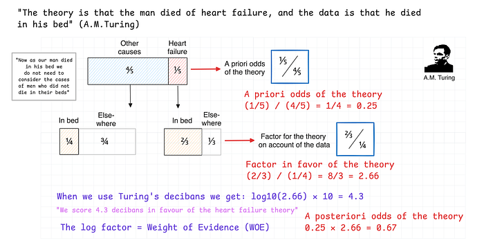
For scoring purposes, Turing proposes to use base-10 logarithm of factors to convert them to “decibans” named after an English town, Banbury. For a more detailed story about Banbury and bans, I recommend this chapter by David MacKay. Decibans were adopted for faster testing, as scores could be added and subtracted, and because larger numbers are easier to handle.
Turing’s work lays the foundation for modern scoring systems, where each input contributes an independent piece of evidence to the final decision. Logarithmic scoring models assign scores to features, with the final score representing the sum of log factors that reflect cumulative evidence. This method forms the backbone of credit scoring as we know it today.
WOE in Credit Scoring
WOE scores allow us to convert raw data into interpretable, additive evidence used in risk decisions.
If you are familiar with credit risk, you might wonder how what we presented above connects with the formulas used in credit risk modeling. In building scorecards, WOE is calculated for each feature-bin combination by taking the ratio of conditional probabilities and then fitting a logistic regression of the form:
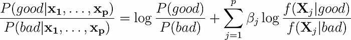
WOE is typically computed using a contingency table, where it represents the logarithm of the ratio between:
- The share of “goods” (e.g., non-defaults) in a bin relative to the total number of goods.
- The share of “bads” (e.g., defaults) in the same bin relative to the total number of bads.
While the order of division (goods-to-bads or vice versa) is not critical in general, credit risk modeling conventionally uses goods-to-bads for logistic regression. You can find an illustrative example here.
Consider a group of bank customers whose credit card usage exceeds 90%. How many of these customers are likely to default?
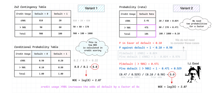
Below I provide a sketch of this calculation (note that I use bads-to-goods ratio as in Turing’s example):

If we look into the group with usage exceeding 90%, we will find 80 out of 100 defaulted customers and 90 of all 900 non-defaulted ones. The factor is then (8/10) / (1/10) = 8.0. This means in this group, we have eight bad loans to a one good loan. A WOE score is then log(8) = log(-0.125) = 2.07.
If we add the log of a priori odds of default (-2.20) to this score, we will get a -0.128. Passing this value to the sigmoid function allows us to obtain a probability of default given usage > 90% equal to 47%. We can also derive this probability by calculating a share of defaulted class within the credit usage group > 90%, which gives the same number.
WOE and Probability
Each WOE score represents a piece of evidence for or against a hypothesis, independent of other features. At Bletchley Park, the focus of scoring was primarily on the scores themselves, without explicitly incorporating prior odds. However, to derive probability estimates, as demonstrated earlier, we must combine the WOE score with the prior odds. WOE acts as a “residual” added to the a priori odds to yield the final probability estimate.
It is important to note that WOE alone cannot determine probability — it must always be interpreted relative to the prior log odds. The final probability is obtained by aggregating the sum of WOE scores across all features and combining them with the prior log odds.
In most applications, logistic regression is used as the final step to compute probabilities. Maximum likelihood estimates (weights) are assigned to WOE scores to produce the final logit and derive probability. However, when assuming the independence of evidence, probabilities can be derived directly by summing the WOE scores across features without the need for logistic regression model.
We can calculate WOE in two ways. The first approach uses a contingency table while the second leverages Bayes factor (see Jack Good’s explanation). As you can see in the sketch below, both methods result in the same factor of 8 we discovered earlier.
WoeBoost
WoeBoost is a new gradient boosting framework inspired by the ideas of Alan M. Turing and his use of log factors (WOE). WoeBoost views each boosting iteration (pass) as an independent contribution of evidence, updating the prior log odds to reflect the final prediction.
Much like the traditional application of using WOE with logistic regression, WoeBoost allows to:
- Handle categorical inputs,
- Enforce business logic with monotonic constraints,
- Handle missing values.
WoeBoost bridges the gap between the predictive power of gradient boosting and the interpretability required in high-stakes domains like finance, healthcare, and law. It also produces calibrated scores, which is a key ingredient of accurate decisions.
In addition, there are two AutoML-like features that can simplify modeling efforts:
- Infer monotonic relationships from data (
infer_monotonicity), - Converge based on early stopping metric reduction (
enable_early_stopping).
In addition, we can perform subsampling of data (useful for large datasets), randomize binning strategies, as well as leverage multi-threading for CPU jobs.
To diagnose models and explain the results, WoeBoost offers a toolkit with custom partial dependence, feature importance, and decision boundary functionality.
How WoeBoost Works
Below I provide a sketch of how WoeBoost works:

1. Initialization
- WoeBoost begins with the prior log odds, representing the baseline log odds of the target outcome (e.g., credit default).
- This value reflects the average event rate in the dataset, with no feature-specific information considered initially.
2. Iterative Evidence Updates
At each boosting iteration:
- Binning of input features is performed using either histograms or quantiles to discretize numerical variables. For categorical variables, unique categories are used as bins.
- Residual averaging for each feature-bin, representing the difference between the observed outcomes and the cumulative predictions from the previous iterations.
- Evidence aggregation by summing residuals for each feature per observation. This is similar to assigning an equal weight of one.
3. Accumulation of Evidence
- After each iteration, the WOE contributions are added to the prior log odds and previous iterations.
- The algorithm converges if the log likelihood loss stops to decrease compared to the previous iterations.
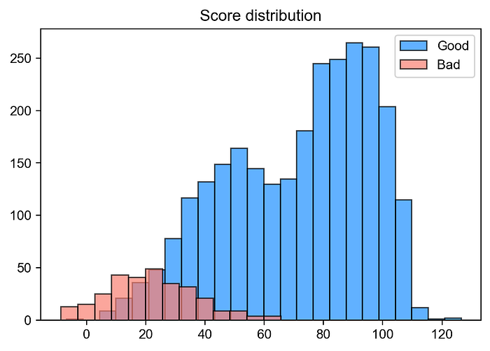
After training, we can use predict_score method to get a distribution of scores (in decibans) to visualize our scoring results. In this example, we see that a score around 40 would allow us to use as a threshold to effectively separate good outcomes from bad ones for classification.
Additionally, we can visualize the results of training in several ways, for example, we can trace the decision boundaries of any two features as the model training progresses. In the chart below, we did not infer monotonic constraints, therefore we see histogram-like patterns.

Other useful features include WoeInferenceMaker which allows you to look into bins taking into account an observed label vector and calculate probabilities, counts of events and non-events, and standard WOE. Additionally, you can use these statistics from each WoeLearner as a stand-alone scoring model following the classical approach. These features are experimental and will be enriched in the future.
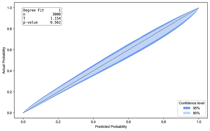
Calibration
Here we rely on PyCalEva package to produce calibration confidence belts for the trained model. This package also contains several calibration tests, like Spiegelhalter’s z-test, which can help with calibration diagnostics.
We can see that the resulting model is well calibrated on the test data. We did not use any parameters, and the model converged automatically.
Below I provide a KL divergence summary between WoeBoost and other algorithms that have proven useful in risk modeling, namely XGBoost, OptBinning, and CatBoost. We run these algorithms with off-the-shelf hyperparameters.
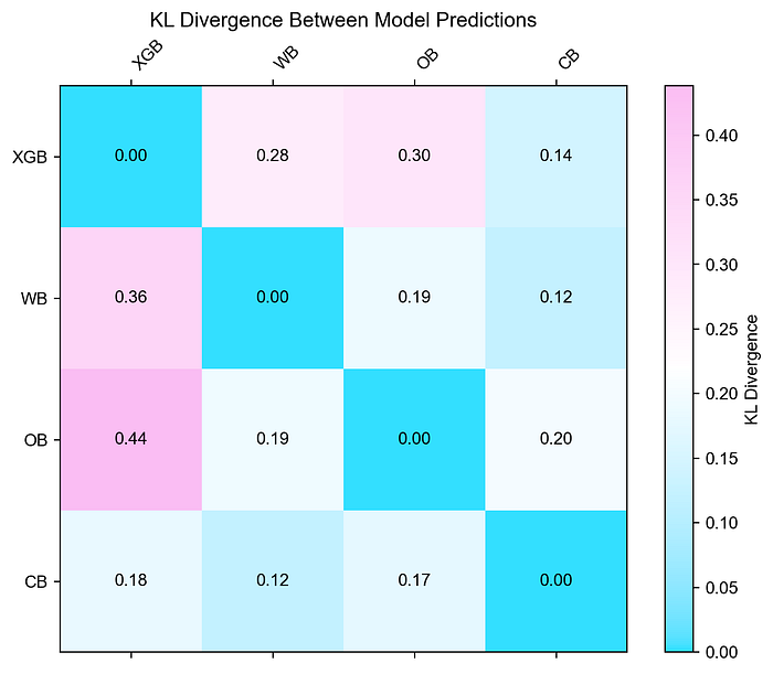
As we can see here, WoeBoost’s predictions are most similar to CatBoost and most dissimilar to XGBoost.
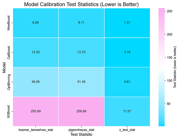
In terms of calibration, WoeBoost ranks first on Hosmer Lemeshow Test, Pigeon Heyse Test, and Spiegelhalter z-test, which shows its practical utility in scoring tasks where calibration is important.
Try WoeBoost
Get started by installing WoeBoost with pip:
pip install woeboostReferences
Alan M. Turing: The Applications of Probability to Cryptography. https://arxiv.org/abs/1505.04714
I. J. Good. Good Thinking: The Foundations of Probability and Its Applications. https://www.jstor.org/stable/10.5749/j.ctttsn6g
N. I. Fisher. A Conversation with Jerry Friedman. https://arxiv.org/pdf/1507.08502